1 Introduction to GW-BSE
- 1.1 Theory
- 1.2 Implementation in BerkeleyGW
  - 1.2.1 Tips for Running Kernel
  - 1.2.1 Tips for Running Absorption
2 Tutorials
- 2.1 Silicon Absorption
3 References

1 Introduction to GW-BSE

1.1 Theory

Si_absorption — Fig. 1: Comparison of the absorption spectrum of bulk Si calculated within the GW plus inter-band transitions approximation (Non-Int.) and GW-BSE approximation (Interacting) with experiment. This figure is taken from Ref. [Deslippe2012].

The GW approximation yields accurate QP energies, but it does not yield accurate optical absorption spectra. For instance, in Fig. 1, which shows optical absorption of bulk Si calculated within the GW approximation and the inter-band transition model compared with experiment, you can see that the experimental spectrum has a different absorption strength from the GW inter-band transition results and has peak-like features, which are not present in the GW spectrum. This difference is not surprising, since GW plus inter-band transitions is a theory designed to describe single-particle excitations, while optical absorption is fundamentally a two-particle process. For instance, you can imagine a photon coming in and exciting a quasi-electron and a quasi-hole, but the quasi-electron and quasi-hole can interact. Thus, the true excitation is not a free quasi-electron and quasi-hole pair but rather a correlated quasi-electron and quasi-hole pair known as an exciton, which can be either a bonafide bound state or resonant (Fig. 2). To good approximation, we can write the exciton state as a linear combination of quasi-electron and quasi-hole states
$|S_{\mathbf{Q}}\rangle =\sum_{vc\mathbf{k}} A^S_{vc\mathbf{kQ}} |v\mathbf{k}\rangle\otimes|c\mathbf{k}+\mathbf{Q}\rangle,$
where $S$ indexes the exciton state; $\mathbf{Q}$ is the exciton’s center-of-mass momentum, and $A^S_{vc\mathbf{k}}$ is the amplitude of the free quasi-electron and quasi-hole pair consisting of an electron in state $|c\mathbf{k}+\mathbf{Q}\rangle$ and an electron missing from state $|v\mathbf{k}\rangle$ .

Fig. 2: Two pictures of excitonic states. The left-hand figure shows a photon with momentum $\mathbf{Q}$ and energy $\omega$ exciting an exciton from the many-body ground state. The excitonic states have an energy vs. center-of-mass momentum $\mathbf{Q}$ dispersion, and depending on the strength of the electron-hole interaction, may have multiple bound states as well as a continuum of states. The right-hand figure illustrates a exciton state as a combination of correlated interband transitions between occupied and unoccupied states in the QP bandstructure. This figure is adapted from Ref. [Cohen2016]

Fig. 2: Two pictures of excitonic states. The left-hand figure shows a photon with momentum $\mathbf{Q}$ and energy $\omega$ exciting an exciton from the many-body ground state. The excitonic states have an energy vs. center-of-mass momentum $\mathbf{Q}$ dispersion, and depending on the strength of the electron-hole interaction, may have multiple bound states as well as a continuum of states. The right-hand figure illustrates a exciton state as a combination of correlated interband transitions between occupied and unoccupied states in the QP bandstructure. This figure is adapted from Ref. [Cohen2016]

For two-particle excitations, we need to introduce the electron-hole correlation function $L$ [Strinati1988]
$L(1,2;1',2') = -G_2(1,2;1',2') + G(1,1')G(2,2').$
Here, the notation $(1)$ represents the combined time, spin, and spatial coordinate; i.e. $(1)=(\mathbf{r}_1,\sigma_1,t_1)$ , and $G_2$ is the two-particle Green’s function. We will also use $(\mathbf{x})$ to refer jointly to the spin and spatial coordinate; i.e. $(\mathbf{x})=(\mathbf{r},\sigma)$ . The electron-hole correlation function obeys a Dyson equation known as the Bethe Salpeter equation (BSE)
$L(1,2;1',2') = L_0(1,2;1',2') + \int d(3456) L_0(1,4;1',3) K(3,5;4,6)L(6,2;5,2').$
Here, $L_0(1,2;1'2')=G(1,2')G(2,1')$ and describes a non-interacting quasi-electron and quasi-hole pair. $K$ is the electron-hole interaction kernel.Following Strinati[Strinati1988] and Rohlfing and Louie[Rohlfing2000], the BSE can be written as an effective eigenvalue problem. In this form the BSE Hamiltonian has the structure
$H^{\mathrm{BSE}}(\mathbf{Q}) = (\varepsilon_{c\mathbf{k}+\mathbf{Q}}^{\mathrm{QP}}-\varepsilon^{\mathrm{QP}}_{v\mathbf{k}'})\delta_{\mathbf{k}+\mathbf{Q},\mathbf{k}'} + \left( \begin{array}{cc} K^{AA}(\mathbf{Q}) & K^{AB}(\mathbf{Q}) \\ K^{BA}(\mathbf{Q}) & K^{BB}(\mathbf{Q}) \\ \end{array} \right),$
where the kernel matrix elements in each block are calculated in the basis of the single-particle orbitals. The off-diagonal blocks ( $K^{AB}$ , $K^{BA}$ ) can usually be neglected as long as the energy of the electron-hole interaction is small compared with the QP gap. Then, the BSE Hamiltonian becomes
$H^{\mathrm{BSE},\mathrm{TDA}}(\mathbf{Q}) = (\varepsilon_{c\mathbf{k}+\mathbf{Q}}^{\mathrm{QP}}-\varepsilon^{\mathrm{QP}}_{v\mathbf{k}'})\delta_{\mathbf{k}+\mathbf{Q},\mathbf{k}'} + K^{AA}(\mathbf{Q})$
This is known as the Tamm-Dancoff approximation (TDA).The BSE kernel is found by taking the functional derivative of the self energy.
$K(3,5;4,6) = \frac{\delta[V_H(3)\delta(3,4) + \Sigma(3,4)]}{\delta G(6,5)}.$
Within the GW approximation for $\Sigma$, the BSE Kernel becomes [Rohlfing1998,Albrecht1998,Rohlfing2000]
$K(3,5;4,6) = -i\delta(3,4)\delta(5^-,6)v(3,6) + i \delta(3,6)\delta(45)W(3^+,4).$
We refer to the first term involving the bare Coulomb interaction as the exchange kernel ( $K^x$ ) and the second term involving the screened Coulomb interaction as the direct kernel ( $K^d$ ).When the spin-orbit interaction is small, the BSE matrix can be block-diagonalized and decoupled into spin-singlet and spin-triplet classes of solution. For the singlet solutions, the BSE kernel is $K^d+2K^x$ . For the triplet solutions, there is no exchange contribution, and the BSE kernel is simply $K^d$ . Only the singlet states are optically bright.Once we have the solutions of the BSE Hamiltonian, we can relate them to the optical spectra. Optical absorption and conductivity are proportional to the imaginary part of the macroscopic dielectric function, $\Im\epsilon_M$ . The macroscopic dielectric function is defined as
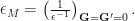
$\epsilon_M = \left(\frac{1}{\epsilon^{-1}}\right)_{\mathbf{G}=\mathbf{G}'=0}.$
Since we are only interested in optical properties, we want to avoid having to calculate and invert $\epsilon^{-1}$ , which is a large matrix. We use the double inversion procedure of Pick, Cohen, and Martin[Pick1970,Hanke1978,Onida2002] to directly obtain $\epsilon_M$ . In this procedure, we replace the Coulomb potential in Fourier space with a modified Coulomb potential, which does not include a long-range contribution. Then, we can construct $\Im \epsilon_M$ from the solutions of the modified BSE
$\Im\epsilon_M(\omega) = \frac{8\pi^2e^2}{\omega^2} \sum_S |\hat{\mathbf{\lambda}}\cdot\langle 0|\mathbf{v}|S\rangle |^2 \delta(\omega-\Omega^S) \\ = \frac{8\pi^2e^2}{\omega^2} \sum_S |\sum_{vc\mathbf{k}} A^S_{vc\mathbf{k}}\hat{\mathbf{\lambda}}\cdot\langle v\mathbf{k}|\mathbf{v}|c\mathbf{k}\rangle |^2 \delta(\omega-\Omega^S)$
where $\hat{\mathbf{\lambda}}$ is the polarization vector, and $\mathbf{v}$ is the velocity operator. We are assuming $\mathbf{Q}\approx 0$ and dropping the $\mathbf{Q}$ index, since the momentum carried by light is very small.
In the independent QP picture (i.e. neglecting excitonic effects), $\Im\epsilon_M$ is becomes
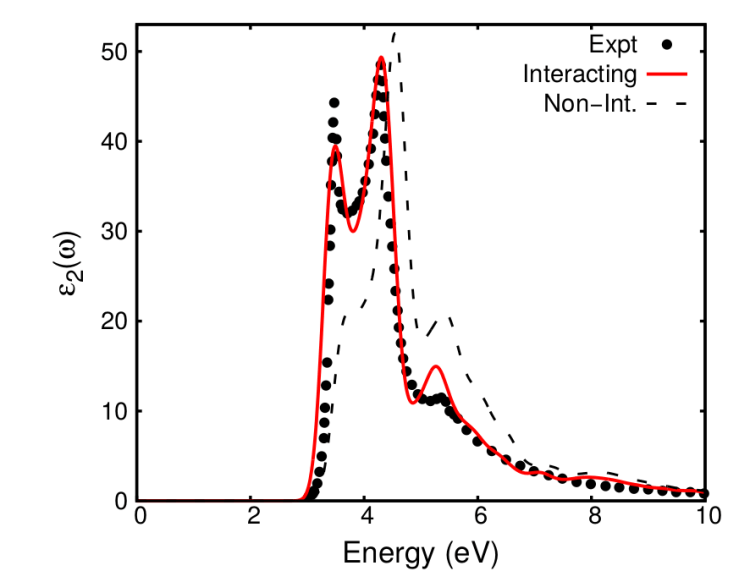
$\Im\epsilon_M = \frac{8\pi^2e^2}{\omega^2} \sum_{vc\mathbf{k}} |\hat{\mathbf{\lambda}}\cdot\langle v\mathbf{k}|\mathbf{v}|c\mathbf{k}\rangle |^2 \delta(\omega-\varepsilon^{\mathrm{QP}}_{c\mathbf{k}} + \varepsilon^{\mathrm{QP}}_{v\mathbf{k}}).$
A comparison of $\Im\epsilon_M$ in the BSE and independent QP inter-band transitions picture is shown in Fig. 1. You can see that including the excitonic effects from BSE results in optical spectra in excellent agreement with experiment.

1.2 Usage in BerkeleyGW

The optical properties of materials are computed in the Bethe-Salpeter equation (BSE) executables. Here the eigenvalue equation represented by the BSE is constructed and diagonalized yielding the excitation energies and wavefunctions of the correlated electron-hole excited states. There are two main executables: kernel and absorption. In the former, the electron-hole interaction kernel is constructed on a coarse k-point grid, and in the latter the kernel is (optionally) interpolated to a fine k-point grid and diagonalized.

First, the kernel executable constructs the direct and exchange kernels as matrices in the basis of electron-hole pairs. The required input files are:

epsmat and eps0mat: dielectric matricees from the epsilon step
WFN_co: mean field wavefunction on a coarse k-grid

The exchange ( $K^x$ ) and direct ( $K^d$ ) matrix elements are
$\langle vc\mathbf{kQ}|K^x|v'c'\mathbf{k}'\mathbf{Q}\rangle = \int d\mathbf{x}d\mathbf{x}' \phi^*_{c\mathbf{k}+\mathbf{Q}}(\mathbf{x})\phi_{v\mathbf{k}}(\mathbf{x})v(\mathbf{r},\mathbf{r}') \phi^*_{v'\mathbf{k}}(\mathbf{x}')\phi_{c'\mathbf{k}'+\mathbf{Q}}(\mathbf{x}') \\ \langle vc\mathbf{kQ}|K^d|v'c'\mathbf{k}'\mathbf{Q}\rangle = -\int d\mathbf{x}d\mathbf{x}' \phi^*_{c\mathbf{k}+\mathbf{Q}}(\mathbf{x})\phi_{c'\mathbf{k}'+\mathbf{Q}}(\mathbf{x})W(\mathbf{r},\mathbf{r}';\omega=0) \phi^*_{v'\mathbf{k}'}(\mathbf{x}')\phi_{v\mathbf{k}}(\mathbf{x}').$
The kernel matrices are output in the `bsemat` file.

1.2.1 Tips for Running Kernel

If the number of CPUs is less than the number of k-points squared ( $N_k^2$ ), $\mathbf{k}$ and $\mathbf{k}'$ pairs are distributed evenly over the CPUs. Thus, if you are using fewer CPUs than $N_k^2$ , you should use a number of CPUs that divides evenly into $N_k^2$ . Similarly, if your number of CPUs is greater than $N_k^2$ and less than $N_k^2\cdot N_c^2$ , your number of CPUs should divide evenly into $N_k^2\cdot N_c^2$ . If you are using more than $N_k^2\cdot N_c^2$ CPUs, the number of CPUs should divide evenly into $N_k^2\cdot N_c^2 \cdot N_v^2$ , where $N_c$ and $N_v$ are respectively the number of valence and conduction bands.
If each MPI task has enough memory to store the entire dielectric matrix, you should use the `low_comm` flag. This minimizes communication and makes the calculation faster.
The kernel executable contains no check-pointing, so make sure to check your output file at the start of your calculation to see if you have enough walltime and memory to finish.
The full list of kernel options can be found here.

The absorption code takes the bsemat file from kernel and constructs the BSE Hamiltonian. The required input files are:

bsemat: kernel matrix
WFN_co: the same coarse grid wavefunction used in the kernel step
eqp_co.dat/eqp.dat (optional): QP energies from sigma on the same k-grid as WFN_co/WFN_fi
WFN_fi (optional): wavefunction on a fine k-grid that can be used to interpolate the kernel matrix elements. This file is not needed if you choose not to interpolate (not recommended) or are studying a system without k-points.
WFNq_fi (optional): wavefunction with a small k-shift with respect to the k-grid of WFN_fi. This is used to calculate the velocity matrix elements, which determine the oscillator strength. This file is not needed if you use choose to use the momentum operator, which neglects the nonlocal parts of the pseudopotential.
epsmat and eps0mat: dielectric matrices from the epsilon calculation

3 References

[Albrecht1998] Stefan Albrecht, Lucia Reining, Rodolfo Del Sole, and Giovanni Onida. Ab Initio calculation of excitonic effects in the optical spectra of semiconductors. Phys. Rev. Lett., 80:4510–4513, May 1998.
[Cohen2016] M.L. Cohen and S.G. Louie. Fundamentals of Condensed Matter Physics. Cambridge University Press, 2016.
[Deslippe2012] Jack Deslippe, Georgy Samsonidze, David Strubbe, Manish Jain, Marvin L. Cohen, and Steven G. Louie. BerkeleyGW: A massively parallel computer package for the calculation of the quasiparticle and optical properties of materials and nanostructures. Comput. Phys. Commun., 183:1269, 201
[Hanke1978] W. Hanke. Dielectric theory of elementary excitations in crystals. Advances in Physics, 27(2):287–341, 1978.
[Onida2002] Giovanni Onida, Lucia Reining, and Angel Rubio. Electronic excitations: density-functional versus many-body Green’s-function approaches.
Rev. Mod. Phys., 74(2):601–659, jun 2002.
[Pick1970] Robert M. Pick, Morrel H. Cohen, and Richard M. Martin. Microscopic theory of force constants in the adiabatic approximation. Phys. Rev. B, 1:910–920, Jan 1970.
[Rohlfing1998] Michael Rohlfing and Steven G Louie. Electron-hole excitations in semiconductors and insulators. Phys. Rev. Lett., 81(11):2312–2315, 1998.
[Rohlfing2000] Michael Rohlfing and Steven G. Louie. Electron-hole excitations and optical spectra from first principles. Phys. Rev. B, 62(8):4927–4944, aug 2000.
[Strinati1988] G. Strinati. Application of the Green’s functions method to the study of the optical properties of semiconductors. Riv. Nuovo Cimento, 11:1, 1988.